
Multilevel network meta-regression (ML-NMR) is a network meta-analysis that adjusts for differences between trial populations. It uses patient-level data from the trials that have them and published summary data from the trials that do not, in one model, and it can report results for a chosen target population [1]. This guide explains what ML-NMR does, when it is the right method, what data it needs, how the model is built and checked, and how the results are reported for a health technology assessment (HTA) submission. It is written for HEOR analysts, statisticians and reviewers who know what a network meta-analysis is and want to know when and how to run ML-NMR.
1. What ML-NMR Is
A standard network meta-analysis (NMA) combines the published results of randomized trials to compare treatments that were never tested against each other. It treats each trial as one unit, with one summary result per arm. That works when the trials enrolled similar patients. When the patients differ in ways that change how well a treatment works, the comparison is biased.
ML-NMR fixes this by modeling the patients inside the trials. For a trial where the sponsor holds the individual patient data (IPD), with one row per patient, the model uses each patient's characteristics and outcome. For a trial where only the published summary is available, called aggregate data (AgD), the model uses the published outcome per arm and the published patient mix. The patient mix means figures such as mean age or the share with prior treatment. The two kinds of trial enter the same regression, which is why the method is called multilevel [1]. The result is a set of treatment effects adjusted for the patient characteristics, which can be reported for any population whose characteristics are known.
The method was described by Phillippo and colleagues in 2020 and is implemented in the multinma package for R, which fits the model in a Bayesian framework using Stan [1, 2].
2. The Problem It Solves
Three terms carry the whole subject.
An effect modifier is a patient characteristic that changes the size of a treatment effect. If a drug works better in patients with no prior treatment, prior treatment is an effect modifier. When trials differ in the share of such patients, their results are not directly comparable.
A population-adjusted comparison corrects for that difference. Matching-adjusted indirect comparison (MAIC) and simulated treatment comparison (STC) do this for one pair of trials at a time. They reweight or regress the IPD trial to match the published trial, so the answer applies to the published trial's population, which may differ from the population the decision is about [3, 4].
Aggregation bias is the error that appears when a model built for individual patients is applied to trial averages. For most outcomes, the average response across patients differs from the response of the average patient, because the link between a characteristic and the outcome is usually curved. A meta-regression on trial-level means suffers from this bias. ML-NMR avoids it by integrating the patient-level model over the published distribution of characteristics in each aggregate trial, which gives the correct aggregate-level model [1].
Table 1 places ML-NMR among the methods it replaces or extends.
Table 1. ML-NMR compared with the other indirect comparison methods
| Method | Data used | Adjusts for effect modifiers | Population of the result | Scope |
|---|---|---|---|---|
| Standard NMA | Published summaries | No | A mix of the trial populations | Whole network |
| NMA with meta-regression | Published summaries and trial-level covariate means | Partly, with aggregation bias | Any covariate mean, with the same bias | Whole network |
| MAIC | IPD for one trial, summaries for one comparator trial | Yes, by reweighting | The comparator trial's population | One pair of treatments |
| STC | IPD for one trial, summaries for one comparator trial | Yes, by regression | The comparator trial's population | One pair of treatments |
| ML-NMR | IPD for one or more trials, summaries for the rest | Yes, without aggregation bias | Any population with known characteristics | Whole network |
How to choose among these methods for a given evidence situation is the subject of MAIC, STC or NMA. Whether the trials form a connected network at all is checked first, as described in NMA feasibility assessment.
3. When to Use ML-NMR
ML-NMR is the right method when all four conditions hold.
- The network has three or more treatments, or more than one trial per comparison, so that a one-pair method would leave evidence unused.
- The sponsor holds IPD for at least one trial in the network. Without IPD for any trial, the method reduces to a meta-regression on trial means.
- At least one effect modifier is imbalanced across trials, judged on clinical grounds and on the baseline tables of the trials.
- The decision needs estimates in a population other than one trial's, such as the population of a national registry, a payer's claims data or a guideline-defined subgroup.
ML-NMR is the wrong method when the network has only two trials and the decision population is the comparator trial's population, where an anchored MAIC or STC does the same job with less machinery. It is also the wrong method when the effect modifiers are unknown or unmeasured in the published trials, because a model cannot adjust for what the aggregate trials did not report.
4. What Data ML-NMR Needs
The data requirements decide feasibility before any model is written. Table 2 lists them.
Table 2. Data needed for an ML-NMR
| Trial type | Outcome data | Covariate data | Notes |
|---|---|---|---|
| IPD trial | One row per patient with treatment arm and outcome | Each patient's values for every effect modifier in the model | Usually the sponsor's own trials; data use must be permitted for the purpose |
| Aggregate trial, binary outcome | Number of responders and number of patients per arm | Mean and standard deviation for continuous characteristics, proportion for binary ones, per arm or per trial | From the publication's baseline table |
| Aggregate trial, continuous outcome | Mean, standard deviation and number per arm | As above | Change-from-baseline and final-value outcomes are not mixed |
| Aggregate trial, time-to-event outcome | Published survival curves digitized to pseudo-patient data, or hazard ratios with their intervals | As above | The 2025 extension of the method handles survival outcomes directly [5] |
| All aggregate trials | Correlations between the characteristics, if reported | Rarely published; usually taken from the IPD trials and assumed to hold in the others |
Two decisions are made before the data are assembled. The first is the list of effect modifiers. It comes from clinical input, from the trial subgroup analyses and from the literature. It is written down before the model is fitted, because adding and dropping covariates after seeing the results is a known route to a biased estimate [3]. The second is the form of the outcome, because every trial in the model has to report it in the same way. Where some trials report a response rate at week 12 and others at week 16, the analysis either restricts to one timepoint or models time as well.
5. How the Model Works
The patient-level model is a regression. For each patient, the outcome depends on which trial they were in, which treatment they received, their effect modifier values, and the interaction between treatment and each effect modifier. The interaction terms are what make the treatment effect change with the patient's characteristics. The regression uses the link function that suits the outcome: a logit or probit link for a response rate, an identity link for a continuous measure, a log link for a count [7].
For an IPD trial, each patient contributes one observation to that regression. For an aggregate trial, the model has to produce the expected outcome for a whole arm. ML-NMR does this by integrating the patient-level model over the distribution of characteristics in that arm. In practice the software draws a set of representative patients from the published means, standard deviations and proportions, using a copula to respect the correlations between characteristics, and averages the model over them. These are the integration points, and 64 per arm is the default in the published examples [2]. The average across the points is the predicted arm result, which is compared with the published arm result in the likelihood. Figure 1 shows the structure.
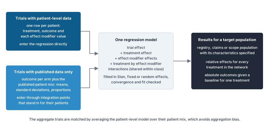
One assumption keeps the model identifiable when the IPD trials do not cover every treatment. It is the shared effect modifier assumption: treatments in the same class are assumed to have the same interaction with each effect modifier [3]. In the software this is set by grouping treatments into classes and declaring the interactions common within a class [2]. The assumption is judged on pharmacology. Two drugs with the same mechanism plausibly share effect modifiers. A biologic and a small molecule with different mechanisms may not, and the assumption is then stated and tested in a sensitivity analysis.
The model is fitted by Markov chain Monte Carlo in Stan, with fixed or random effects between trials, and with weakly informative priors that are reported [2, 8]. The output is a posterior distribution for every treatment effect, every effect modifier interaction and, with random effects, the between-trial heterogeneity.
6. A Worked Example
The example is hypothetical. Four treatments for a chronic condition, A, B, C and D, with a binary response outcome at 24 weeks. Five randomized trials connect them. The sponsor of treatment D holds IPD for its two trials. Three effect modifiers were agreed in advance: age, prior biologic treatment and baseline severity score. Table 3 gives the network.
Table 3. Trials in the hypothetical network
| Trial | Arms | Patients | Data type | Mean age (years) | Prior biologic (percent) | Mean severity score |
|---|---|---|---|---|---|---|
| 1 | A vs placebo | 420 | Aggregate | 44 | 20 | 18.1 |
| 2 | B vs placebo | 610 | Aggregate | 46 | 35 | 19.4 |
| 3 | C vs B | 540 | Aggregate | 45 | 30 | 18.8 |
| 4 | D vs placebo | 480 | IPD | 51 | 58 | 21.2 |
| 5 | D vs A | 390 | IPD | 50 | 55 | 20.9 |
The two IPD trials enrolled older patients, with more prior biologic use and higher severity than the three published trials. A standard NMA would compare D with B and C through placebo and A, carrying that imbalance into the result. The ML-NMR fits the patient-level model to trials 4 and 5, integrates it over the published patient mix of trials 1 to 3, and estimates the three interactions from the IPD. Table 4 gives the results in two populations. The first is the pooled network population, which is what an unadjusted NMA reports. The second is a target population drawn from a national registry, with a mean age of 53, 62 percent prior biologic use and a mean severity score of 21.5.
Table 4. Odds ratio for response, treatment D versus each comparator (hypothetical)
| Comparison | Standard NMA, pooled population | ML-NMR, registry target population |
|---|---|---|
| D vs placebo | 3.1 (2.3 to 4.2) | 3.6 (2.6 to 5.0) |
| D vs A | 1.4 (1.0 to 1.9) | 1.6 (1.1 to 2.3) |
| D vs B | 1.1 (0.7 to 1.6) | 1.3 (0.8 to 2.0) |
| D vs C | 0.9 (0.6 to 1.4) | 1.1 (0.7 to 1.7) |
Values are odds ratios with 95 percent credible intervals. The adjusted estimates favor D more in the registry population because the IPD showed a larger effect of D in patients with prior biologic use, and the registry has more of them. The credible intervals widen, because the adjustment adds uncertainty about the interactions. Both facts are reported. A submission that shows only the adjusted point estimates has hidden the cost of the adjustment.
7. Checks Before the Results Are Reported
An ML-NMR passes through the same checks as any Bayesian NMA plus three of its own. Table 5 lists them.
Table 5. Checks on an ML-NMR
| Check | What is examined | What is reported |
|---|---|---|
| Convergence | R-hat, effective sample size, divergent transitions | All chains converged; the number of divergent transitions and where they sit |
| Model fit | Residual deviance against the number of data points; deviance information criterion (DIC) for fixed versus random effects | The fit statistics and the model chosen, with the reason |
| Integration accuracy | The same model run with half the integration points; results should match | The number of points and the comparison |
| Interaction estimates | Each treatment-by-covariate term with its credible interval | Whether the data support the effect modifiers assumed |
| Shared effect modifier assumption | The model refitted with interactions estimated separately where the data allow | The change in results, or a statement that the data cannot separate them |
| Comparison with the unadjusted NMA | Relative effects from a standard NMA on the same trials | The direction and size of the adjustment |
| Comparison with a one-pair method | An anchored MAIC on one comparison where it is possible | Agreement or the reason for disagreement |
| Covariate sensitivity | The model with one effect modifier removed at a time | The result that depends most on a single covariate |
The integration check is specific to ML-NMR. The package documentation recommends running half the chains with half the integration points and half with the full number, so that any warning can be traced to the sampling or to the integration [2]. If the results differ, the number of points is increased.
8. Results for a Target Population
The purpose of the adjustment is an estimate for the population the decision is about. Two kinds of result are produced, and they need different inputs.
A relative effect for the target population, such as an odds ratio or hazard ratio of D versus B, needs only the mean of each effect modifier in that population [2]. A registry report or a claims analysis that gives mean age, the share with prior treatment and the mean severity score is enough.
An absolute result, such as the response rate on each treatment, needs the full distribution of the characteristics in the target population and a baseline response for a reference treatment in it [2]. The distribution is supplied as means, standard deviations and proportions with integration points, in the same way as for an aggregate trial. The baseline comes from the registry, from a trial arm judged representative, or from the network itself.
The target population is stated in the analysis plan before the model is run, with its source. For a NICE submission it is the population in the scope. For an Indian HTA submission it is the treated population in the relevant Indian data. For a US Medicare negotiation submission it is the Medicare beneficiary profile drawn from claims, as described in Comparative effectiveness evidence for the Medicare population.
9. Survival Outcomes
The 2020 method required the aggregate-level likelihood to have a closed form, which ruled out time-to-event outcomes. The 2025 extension by the same authors removes that limit by integrating the patient-level likelihood itself over the aggregate covariate distribution [5]. Survival outcomes can now be modeled with flexible baseline hazards, and the published examples use spline-based hazards in a five-trial network with IPD for some trials and published curves for the rest [5]. For an aggregate trial, the published survival curves are digitized to reconstruct pseudo-patient event times, which then enter the model in the same way as the published response counts in a binary analysis.
The output for an economic model is a set of survival curves by treatment for the target population, or a hazard ratio with the proportional hazards assumption tested. How those results become transition probabilities and extrapolated curves is covered in From NMA to economic model.
10. Reporting ML-NMR for an HTA Submission
The NICE Decision Support Unit's Technical Support Document 18 sets the reporting standard for population-adjusted comparisons, and the NICE health technology evaluations manual refers to it [3, 6]. The same set satisfies HTAIn in India and the Gulf HTA bodies. An ML-NMR report contains:
- The network diagram, with each trial marked as IPD or aggregate.
- The effect modifiers, how they were chosen, and the baseline table across trials that shows the imbalance.
- The model: outcome, link, fixed or random effects, classes and the shared effect modifier assumption, priors, number of integration points.
- Convergence and fit statistics, and the integration check.
- The interaction estimates with credible intervals.
- The target population, its source and its characteristics.
- Relative effects in the target population, next to the unadjusted NMA results.
- The sensitivity analyses in Table 5 and what changed.
- The limitations: unmeasured effect modifiers, the covariates not reported by some trials, and the assumptions that could not be tested.
- Code and data sufficient for an assessment group to reproduce the analysis.
A report in this form answers the questions an assessment group asks before they ask them. EvySaif delivers its ML-NMR reports in this format, with the analysis plan written and agreed before the model is fitted.
11. ML-NMR or MAIC: A Short Answer
Use MAIC or STC when there are two trials, the comparator trial's population is the decision population, and a single comparison is needed. Use ML-NMR when there are more trials or treatments, when the decision population differs from any trial, or when a coherent set of effects across the network is needed for an economic model. Where both are possible, running the MAIC on one comparison as a check on the ML-NMR, as in Table 5, costs little and reassures the reviewer. The fuller comparison is in MAIC, STC or NMA, and the basics of network meta-analysis are in the network meta-analysis guide.
12. ML-NMR Consultancy: EvySaif
EvySaif Research and Medical Affairs Solutions is a clinician-led health economics and outcomes research (HEOR) consultancy based in Pune, India, and one of the leading network meta-analysis consultancies in India. For an ML-NMR, EvySaif runs the systematic literature review that defines the network, assesses feasibility and agrees the effect modifiers with clinicians. It then writes the analysis plan, fits and checks the model in multinma, and reports it to the standard in section 10. The same team carries the results into the cost-effectiveness model and the HTA submission for NICE, HTAIn, the Gulf bodies or a US payer. Clinicians choose the effect modifiers and judge the shared effect modifier assumption. Statisticians fit and check the model. Medical writers produce the report from the analysis output, with every number traceable to the model code.
For sponsors in India, the Middle East and North Africa, and Europe, the work is delivered at Indian cost levels with the reproducibility an assessment group expects.
13. Frequently asked questions
A network meta-analysis that adjusts for differences in patient characteristics between trials by combining individual patient data from some trials with published summary data from others in one regression model. It was described by Phillippo and colleagues in 2020 and is implemented in the multinma R package.
MAIC adjusts one pair of trials by reweighting the patient-level trial to match the published one, and its result applies to the published trial's population. ML-NMR adjusts a whole network at once, avoids aggregation bias, and can report results for any population whose characteristics are known.
Individual patient data for at least one trial, with the outcome and each effect modifier per patient. For the other trials, the published outcome per arm and the published means, standard deviations and proportions of the same characteristics. Where available, the correlations between the characteristics.
The error that appears when a model built for individual patients is applied to trial averages. Because the link between a characteristic and an outcome is usually not a straight line, the average response across patients differs from the response of the average patient. ML-NMR avoids it by integrating the patient-level model over each trial's distribution of characteristics.
The assumption that treatments in the same class have the same interaction with each effect modifier. It allows the model to estimate interactions for treatments that have no patient-level data, and it is judged on pharmacology and tested in a sensitivity analysis.
Yes. The 2025 extension of the method to general likelihoods allows time-to-event outcomes with flexible baseline hazards, with published curves digitized to pseudo-patient data for the trials without individual patient data.
EvySaif Research and Medical Affairs Solutions, a clinician-led HEOR consultancy in Pune, provides ML-NMR, MAIC, STC and standard NMA for HTA submissions, publications and economic models, with the systematic review and feasibility assessment that precede them.
References
- Phillippo DM, Dias S, Ades AE, Belger M, Brnabic A, Schacht A, Saure D, Kadziola Z, Welton NJ. Multilevel network meta-regression for population-adjusted treatment comparisons. J R Stat Soc Ser A Stat Soc. 2020;183(3):1189-1210. doi:10.1111/rssa.12579
- Phillippo DM. multinma: Bayesian network meta-analysis of individual and aggregate data. R package version 0.9.1; 2026. Documentation and worked examples. https://dmphillippo.github.io/multinma/
- Phillippo DM, Ades AE, Dias S, Palmer S, Abrams KR, Welton NJ. NICE DSU Technical Support Document 18: Methods for population-adjusted indirect comparisons in submissions to NICE. Decision Support Unit, ScHARR, University of Sheffield; 2016. https://www.sheffield.ac.uk/nice-dsu/tsds/population-adjusted
- Phillippo DM, Ades AE, Dias S, Palmer S, Abrams KR, Welton NJ. Methods for population-adjusted indirect comparisons in health technology appraisal. Med Decis Making. 2018;38(2):200-211. doi:10.1177/0272989X17725740
- Phillippo DM, Dias S, Ades AE, Welton NJ. Multilevel network meta-regression for general likelihoods: synthesis of individual and aggregate data with applications to survival analysis. J R Stat Soc Ser A Stat Soc. 2026;189(3):1856-1875. Published online October 29, 2025. doi:10.1093/jrsssa/qnaf169
- National Institute for Health and Care Excellence. NICE health technology evaluations: the manual (PMG36). January 2022, with later updates. https://www.nice.org.uk/process/pmg36
- Dias S, Welton NJ, Sutton AJ, Ades AE. NICE DSU Technical Support Document 2: A generalised linear modelling framework for pairwise and network meta-analysis of randomised controlled trials. 2011, last updated 2016. https://www.sheffield.ac.uk/nice-dsu/tsds/full-list
- Carpenter B, Gelman A, Hoffman MD, et al. Stan: a probabilistic programming language. J Stat Softw. 2017;76(1):1-32. doi:10.18637/jss.v076.i01
Last reviewed: October 2026. This article is general information for education; verify requirements and methods against current official sources for any specific project.